The use of interactive computer models as a means of increasing the motivation of schoolchildren in the study of physics.

In my experience, I use modern computer technologies and interactive models in conjunction with traditional teaching methods to increase the motivation for learning physics.
Teaching physics at school implies the constant support of the course with a demonstration experiment. However, in a modern school, conducting experimental work in physics is often difficult due to a lack of study time and the lack of modern material and technical equipment. With the advent of computer technology, it became possible to supplement the experimental part of the physics course and significantly increase the effectiveness of the lessons. The use of computers in physics lessons turns them into a real creative process, allows you to implement the principles of developmental education. It is possible to select the necessary material, present it clearly, clearly and accessible.
When using it, you can isolate the main thing in the phenomenon, cut off secondary factors, identify patterns, repeatedly conduct a test with variable parameters, save the results and return to your research at a convenient time. In addition, a much larger number of experiments can be carried out in the computer version. This type of experiment is implemented using a computer model of a particular law, phenomenon, process, etc. Working with models opens up enormous cognitive opportunities for students, making them not only observers, but also active participants in ongoing experiments.
Interactive learning uses:
Computer models are programs that allow you to simulate physical phenomena, experiments or idealized situations encountered in tasks on a computer screen.
Virtual laboratories are more complex computer programs that provide the user with much more options than computer models.
The work of students with computer models and laboratories is extremely useful, as they can set up numerous virtual experiments and even conduct small studies. Interactivity opens up huge cognitive opportunities for students, making them not only observers, but also active participants in ongoing experiments.
Since interactive learning is the most modern education, a hypothesis is put forward: through the use of modern computer technologies, the motivation of schoolchildren to study physics should increase. After all, the level of formation of motivation is an important indicator of the effectiveness of the educational process. The use of modern technologies in the study of physics should contribute to solving this problem.
I have been using modern information technologies at school and after school hours since 2003, and with the advent of modern computer equipment and Internet connections at school, the possibilities of organizing and conducting a physics lesson corresponding to the level of the 21st century have expanded even more. Increasingly, in my lessons I try to use an interactive physical experiment, research and laboratory forms of educational activity.
Means of increasing the motivation of schoolchildren in the study of physics
I consider the following forms of work:
lesson, with the creation of a problem situation at its various stages;
using computer testing;
extracurricular work on the implementation of projects and research using Internet resources and training programs.
I use the following pedagogical methods:
- theoretical: analysis of pedagogical, methodological and special literature on the research problem;
- general scientific: pedagogical observation, conversations with schoolchildren, analysis of the results of students' activities, study of computer software products intended for teaching physics at school, study and analysis of the experience of using information technology tools in teaching schoolchildren;
- statistical: processing the results of pedagogical experience.
The task of the teacher is precisely to ensure the emergence, preservation and predominance of the motives of educational and cognitive activity.
Let's start with such an incentive as the novelty of the educational material and the nature of cognitive activity. The new must build on the old. At the beginning of the lesson, in order to update the knowledge of schoolchildren, I conduct physical dictations, increasingly using multimedia products.
The main methods of organizing work with students are conversation, observation, experience, practical work with a predominance of the heuristic nature of the cognitive activity of students. These methods provide the development of research skills, abilities, teach them to make new decisions on their own.
The main form of learning activity is a lesson where I try to create a situation of success for each student, using reproductive, training and final reinforcement, as well as a theory survey.
In my work I rely on the following didactic principles:
individualization and differentiation of education;
principle of creativity and success
principle of trust and support
the principle of involving children in the life of their social environment.
The technological component (methods and techniques of teaching) should, in my opinion, meet the following requirements:
dialogue;
activity-creative character;
focus on supporting the individual development of the child;
providing him with the necessary space for making independent decisions, creativity, choice.

1

The consequence of the recent situation in the country's economy is the growing role of science and engineering education. At the same time, it has not yet become prestigious, school graduates still prefer humanitarian areas of training. To eliminate the existing disproportion, it is necessary to use classical and new tools to develop students' interest in scientific and technical creativity and engineering. In particular, attention should be paid to the introduction into the system of secondary education of mechanisms for the formation of empirical thinking in schoolchildren and the ability to conduct an educational experiment. In this aspect, the possibilities of interactive computer models and simulators in the study of physics are discussed. It is shown that real and computer experiments are not antagonists, but, on the contrary, complement each other and mutually reinforce the achieved learning effect.

mathematical and computer modeling

interactivity

cognitive activity

physical experiment

1. Bayandin D.V. Education in physics based on modeling computer systems // School technologies. - 2011. - No. 2. - P. 105–115.

2. Bayandin D.V. Classification of interactive computer models and the structure of the process of cognition in physics // Modern problems of science and education. - 2013. - No. 2. - P. 311. - URL: www..09.2014).

3. Mostepanenko M.V. Philosophy and physical theory. - L. : Nauka, 1969. - 240 p.

4. Ospennikova E.V. The use of information and communication technologies in teaching physics. - M. : BINOM, 2010. - 655 p.

5. Razumovsky V.G., Maier V.V. Physics at school. Scientific method of cognition and learning. - M. : VLADOS, 2004. - 463 p.

The situation in the economy and in society as a whole, which has developed over the past year and a half in connection with the economic sanctions of the West, has demonstrated the fallacy of the course towards the production of "qualified users" of imported developments, technologies and equipment by the education system - instead of educating our own engineers capable of creating new technologies and equipment on one's own. In this regard, the role of natural science and engineering education should grow in the coming years. However, over the past two decades, a steady orientation of school graduates to receive economic, legal and other humanitarian education has been formed. Young people for the most part want to manage - finance, enterprises, political and social spheres, while there are absolutely not enough of those who want and can develop and produce high-tech products both in the form of goods and in the form of services (which today include medicine and education).

Of course, this situation in the education system can change only as a result of well-thought-out and coordinated actions of the state and society, and not in the form of a short campaign, but in the form of a long-term "new educational policy" that is radically different from that carried out over the past fifteen years.

One of the ways to revive students' interest in natural science education, scientific and technical creativity and engineering is to introduce into the system of secondary education mechanisms for the formation of empirical thinking in schoolchildren and the ability to conduct an educational experiment. In this case, both classical and new tools for developing this interest should be used. An example of a successful innovation is the introduction of robotics into the curriculum of many schools. As for computer technologies, the use of their potential remains insufficiently effective.

There is still a widespread point of view among methodologists that a computer model is not a full-fledged replacement for real objects and phenomena and therefore cannot be useful for the development of students' empirical thinking. As far as the first part of this statement is plausible (to the discussion of which we will return later), so the second is doubtful. We believe that it is quite possible to talk about the formation of the elements of empirical thinking and the skills necessary for conducting an experiment on the basis of interactive computer models and simulators, although, of course, the leading role in this process belongs to a real laboratory experiment.

Traditionally, in empirical research, the following stages are distinguished, which are associated, among other things, with empirical thinking:

1) observation and experiment - a means of obtaining experimental data;

2) analysis and synthesis of results - a means of identifying relationships and systematizing data;

3) generalization of experimental data, the formation of new empirical concepts and laws (with subsequent verification), which make it possible to further explain the phenomenon under study and predict the behavior of the system.

The second and third stages are fully implemented in the model experiment, except for what is analyzed and generalized: the problem of the very procedure for obtaining experimental data remains - if we are talking about computer simulation of a real experimental setup. The first stage of research suffers the most during such a simulation experiment: the sensual side of the process of cognition is depleted, the connection with objective reality is broken. These losses are irreplaceable at the stages of designing (assembling) the experimental setup and actually performing observations and measurements. However, the first stage also includes the stages of formulating the research problem, putting forward and substantiating a hypothesis, on the basis of which the problem can be solved, determining the purpose of the experiment and the procedure for conducting it. If a computer system does not just imitate a real installation, but models some complex phenomenon at a sufficiently high level of abstraction (for example, the establishment of chaos in a system of many particles), then the stage of obtaining data by measurements on a computer model becomes full-fledged, and educational research approaches scientific research. .

Interactive educational models, as well as research models, have certain epistemological functions that determine their didactic and methodological functions. The didactic functions of educational models are associated with the possibilities of their use as a means of visualization in the presentation of knowledge, as a means of developing cognitive skills and skills formation, as well as a means of controlling the level of knowledge and skills of students. The main methodological function of models, formulated in the same work, is the formation of the experience of educational research in schoolchildren, during which subjectively new knowledge is obtained, and the model experiment acts as a method of cognition.

The refraction of the process of scientific knowledge in the educational process is also discussed in the educational publication. Like a real experiment, computer simulations support important steps in educational research. It can be used to:

• to observe, classify and generalize facts, including noticing the similarities and patterns of results;
• interpret data;
• give an explanation of the observed phenomena and put forward hypotheses;
• plan a model experiment to test the hypothesis and conduct it;
• draw conclusions and conclusions based on the research.

One of the important signs of the formation of empirical thinking is the ability to think over the tactics of conducting an experiment, which would fully, but economically in terms of the required efforts, allow solving the research problem. And in this sense, work with a physical installation and with a computer model adequate to it within the framework of the task in hand is similar and practically equally useful. In both cases, the most important are: a) the mental processes taking place in the student's brain; b) the technical capabilities of the “laboratory stand” for testing and, if necessary, correcting the research hypothesis, correcting errors due to operational feedback provided by measuring instruments or the model interface. At the same time, a real laboratory stand, of course, is much richer in its properties and their manifestations than a virtual stand imitating it, but for studying a number of issues, including research tactics, this may not be essential.

The most indicative for illustrating the foregoing are model experiments that make it possible to obtain at the output not a qualitative dependence, even if illustrated by a graph, but a quantitative one, expressed by a formula or a set of numerical values ​​specific to a given situation.

An example of a situation, consideration of which is useful for mastering the ability to plan an experiment, is the classical problem of throwing a body at an angle to the horizon over an inclined plane - “throwing uphill”. This task is included as an independent element, for example, in the “Inter@active Physics” modeling environment (Institute of Innovative Technologies, Perm), but can also be considered on models of a number of other electronic publications for educational purposes.

Let the model allow you to set before the throw (or shot) the angle j of inclination of the "underlying surface" and the angle a between the initial velocity vector of the body and the horizontal, and also to fix the displacement L of the body along the plane at the moment of falling on it (Fig. 1). In this case, the purpose of conducting a model experiment can be to find the dependence amax(j) - the value of the angle of throw, at which the flight range is maximum, on the value of the angle of inclination of the plane.

Rice. 1. Model experiment: the dependence of the flight range of the body on the angle of throw and the angle of inclination of the underlying surface.

Independent planning by students of an appropriate study based on a computer model requires certain skills and experience in this kind of work. A student who does not have the skills to conduct an experiment (whether physical or numerical) often does not even understand that the initial conditions cannot be changed randomly, you need to think through the system - for example, in our case, you should not change the throwing speed. The specifics of working with computer models are usually clarified either through instructions for their study (such as the order of laboratory work), or in the course of problematic conversations that the teacher conducts with the class. For the problem under discussion, the basis of the work plan and a kind of hint can be the order of the model experiment when a body is thrown over a horizontal surface (j=0). His idea is to start the experiment with a small value of the angle a, and then continue throwing, each time increasing the throwing angle by the same amount, for example, by 5º. It is found that the maximum flight range is achieved at a throw angle of 45º, and pairs of angle values ​​that add up to 90º lead to the same flight range.

It remains for the student to figure out that in the case of an inclined "underlying surface" it is necessary to conduct a series of similar experiments with different values ​​of the angle j, determining for each of them the corresponding amax. For further analysis of the results, the pairs of values ​​j and amax should be entered in the table; it is desirable to build a graph illustrating the discovered dependence. Further, it should be noted that the dependence is linear, and write it in the form of the desired function: amax=45º+j/2.

Note that the skill of mathematical recording of this kind of dependencies according to the table or according to the schedule can be practiced using an interactive computer simulator. The same applies to the ability to design the structure of data tables, which is an element of the culture of conducting an experiment. Since from the point of view of physics this is mainly a technical issue, an operational skill, it can be practiced within the framework of a computer simulator not only on the basis of a physical experiment, but also on the basis of a simulation model and even, to save time, a video recording of an experiment or animation. Another number of simulators can be useful for mastering the procedures for taking readings of measuring instruments and assessing the associated errors, recording the result of an experiment in the form of a confidence interval with reasonable accuracy, and not with 8-10 significant figures that a calculator gives. The expert system of the interactive simulator monitors the student's mistakes in the course of work and responds to them in context.

According to our observations, the use of a computer is effective precisely in the development of elementary skills. However, of course, stages of learning are needed, at which all the skills and abilities are included in the “solid” process of conducting the experiment, and here the experiment should no longer be virtual, but real. Thus, computer simulators relieve the teacher of routine work - repeated explanation and control of basic skills and abilities - and allow him to focus on more complex, creative, algorithmically difficult moments. To use such simulators in principle or not is the decision of a particular teacher; it is up to the developer of software and methodological support to offer the very possibility of using them.

Let us now touch on two points related to the problem of the reliability of the results of mathematical modeling: 1) the adequacy of the model of the object under study and 2) the adequacy of the numerical method for solving its system of equations.

The purpose of any model is, first of all, to help the researcher understand this or that natural phenomenon. On the other hand, it is assumed that the simulation results and their logical consequences make it possible to predict the behavior of an object under given (but, as a rule, limited in its diversity by some limits) conditions. If at least some variants of these conditions are realizable in a laboratory or full-scale experiment, it is necessary to compare (directly or indirectly) the experimental data and calculation results; in other words, it is necessary to test the model. The agreement between the experimental and calculated information speaks in favor of the constructed model. On the contrary, significant discrepancies that cannot be attributed to experimental errors, or the inability to interpret the simulation results in terms of experimental data, mean that the model is not adequate, suitable for describing the objective world and must be improved. The more situations are studied in which the model was able to correctly reproduce reality, the more reason it can be used to describe the corresponding effects in similar conditions. However, any, relatively speaking, "interpolation", and even more so "extrapolation" to an unexplored area of ​​conditions, is associated with a certain risk. The same applies to models, the real prototype of which, for some reason, is not suitable or not available for manipulation. In any case, each model has a certain area of ​​applicability, one can speak of adequacy only within this area, and it is up to the researcher to make sure not to go beyond its boundaries.

Now about the adequacy of the numerical method. In computational mathematics, a significant number of methods have been developed for the numerical solution of the problem of integrating systems of differential equations under given initial conditions (the Cauchy problem). These methods have different characteristics, first of all - the accuracy and volume of calculations. The calculation error or error when using a specific numerical method consists of a methodological error (inaccuracy of the algorithm itself, caused, for example, by cutting off members of an infinite series) and a rounding error caused by a limited number of digits (the finite length of a machine word). Therefore, the nature of error accumulation and propagation with an increase in the number of steps significantly depends on the chosen method that implements this method of the algorithm.

Returning to the question of the correctness of replacing real objects and phenomena by a computer model, we note that the model is not obliged to describe all aspects of the phenomenon and the variants of the course of events associated with them. That is, these qualities are good in themselves, especially if we are talking about a model constructor, on the basis of which a wide class of tasks is supposed to be solved, and a specific laboratory bench based on this constructor does not turn out to be “unbearable” in terms of computational speed and interface complexity. However, if we are talking about a separate laboratory work, it is enough that the model only corresponds to the purpose of the experiment. In the example above, there is also no need for a complex model. For example, the model shown in Figure 1 describes multiple bounces of a ball from an inclined plane in a viscous medium, since it is built on the basis of a very universal constructor, the elements of which contain the equations of motion and the procedure for their integration for a spatial region with variable properties of the medium inside it and on its boundaries. However, these possibilities are not used in the laboratory work, so a model built on the simplest kinematic equations or even a parabola equation, the coefficients in which are calculated from the initial conditions of motion, would be completely sufficient.

Another example of a computer model that makes it possible to obtain a formula as a result of its study is the Wheatstone bridge. The purpose of the study may be to clarify the conditions for the balance of the bridge arms (lack of current in the galvanometer). Figure 2 shows the interface of such a model: in the initial state, all resistances are the same, but can be changed by the user during the experiment. First, students find that the balance is maintained if the resistance of two adjacent bridge arms is changed by the same number of times. To generalize this result, to understand that the values ​​of all four resistances can be different, a student with insufficiently developed research skills may need to be encouraged (using the text of the instruction, in the course of a dialogue with a teacher or an expert system). The result of the study is the known proportion of the species: R1/R3 = R2/R4. The advantage of the computer model in this case is the ability to consider a large number of situations in a short time, on the basis of which it is possible to analyze the results and draw a conclusion. After studying the physical system in its model version, students better perceive the theoretical explanation of the pattern found.

Rice. 2. Model experiment: finding out the balance condition of the Wheatstone bridge

Do vehicle simulators or industrial plant simulators replace the corresponding reality? Of course they don't replace it. However, they allow you to prepare for the perception of this reality, to “think” yourself in a similar situation. Similarly, a real experiment cannot be replaced in the educational process by computer technologies, but with a well-thought-out methodology, the latter can serve as an additional tool, a means of teaching influence, which allows you to save time and efforts of the teacher, develop skills and abilities, including those associated with experimental activities, and even develop empirical thinking.

Reviewers:

Ospennikova E.V., Doctor of Pedagogical Sciences, Professor, Head. cafe multimedia didactics and information technologies of education of the Perm State Humanitarian and Pedagogical University, Perm;

Serova T.S., Doctor of Pediatric Sciences, Professor of the Department of Foreign Languages, Linguistics and Translation, Perm National Research Polytechnic University, Perm.

Bibliographic link

Bayandin D.V. INTERACTIVE COMPUTER MODELS AND FORMATION OF ELEMENTS OF EMPIRICAL THINKING // Modern problems of science and education. - 2015. - No. 5.;
URL: http://science-education.ru/ru/article/view?id=21814 (date of access: 02/01/2020). We bring to your attention the journals published by the publishing house "Academy of Natural History"

^^ 1 ELECTRONIC LEARNING RESOURCES:

>/ DEVELOPMENT AND METHODOLOGY OF APPLICATION IN TRAINING

UDC 004.9 BBK 420.253

YES. Antonova

PRINCIPLES OF DESIGNING INTERACTIVE LEARNING MODELS OF A PHYSICAL EXPERIMENT USING THE MAXIMUM REALISTIC INTERFACE TECHNOLOGY

The content of the project activity of students on the development of interactive models of a school physical experiment, implemented in the technology of the most realistic interface, is considered. The main principles for designing models of this type are determined: realistic visualization of the experimental setup and its functionality, quasi-realistic actions with the elements of the setup and physical objects under study, ensuring a high level of model interactivity and compliance of its scenario solutions with the methodology of experimental research, focusing on the formation of students' generalized skills in working with computer model. The importance of the relationship between methodological and technological approaches to the design of educational interactive models is substantiated.

Keywords: teaching physics, physical experiment, experimental skills, interactive model, principles of designing educational models of a physical experiment

Mastering the course of physics in secondary school should be based on numerous observations and experiments (both demonstration and laboratory). The implementation of experiments allows students to accumulate a volume of factual material sufficient for systematization and meaningful generalization and acquire the necessary practical skills. Empirical knowledge obtained in the course of observations and experiments forms the necessary basis for the subsequent theoretical understanding of the essence of the studied natural phenomena.

Unfortunately, the stage of empirical knowledge associated with conducting experiments is very limited in time in high school. The amount of relevant practical work performed by students is also small (a demonstration physical experiment is mainly work “by the hands of a teacher”, a laboratory experiment is few, and home experiments are rarely included by teachers in the content of training). The modern technical environment also has a negative impact on this situation. It does not encourage students to observe natural phenomena and study the features of their course. "The reason for this is" packaging "

© Antonova D.A., 2017

these phenomena into complex technical devices that carefully surround us and invisibly satisfy our needs and interests.

The resources of the virtual environment can be considered as an important additional tool for training students in the field of experimental research methodology. First of all, attention should be paid to improving and expanding the base of video materials (reporting, staged) related to natural physical experiments (observations and experiments). A realistic video sequence contributes to the expansion of the empirical horizons of students, makes physical knowledge contextual and in demand in practice. Useful in teaching are photographs and objects of static and interactive computer graphics, revealing the content and stages of setting up various physical experiments. It is necessary to develop educational animation illustrating the peculiarities of the course of the studied phenomena, as well as the operation of various objects of technology, including physical devices.

The subject of special interest is the objects of the virtual environment, simulating the educational physical experience and practical actions of the user with devices and materials for its implementation. The complex of unique features of this learning environment (intelligence, modeling, interactivity, multimedia, communication, performance) allows developers to create these objects at a high quality level. Interactive educational models of a physical experiment are in high demand in the educational market, so it is necessary to constantly work to fill the subject environment with models of this type.

The search for approaches to the creation of virtual models of physical experiments and their first implementation date back to the early 2000s. During this period, such models were, as a rule, the simplest animation of natural physical processes or stages of performing a physical experiment to study them. Later, models appeared with a button-animated interface that allows the user to change the parameters of the model and observe its behavior. Soon, the visualization of the external signs of phenomena began to be supplemented by the visualization of the mechanisms of their occurrence in order to illustrate the provisions of one or another physical theory explaining these phenomena. A feature of the visual representation of physical experiments in a virtual environment in this period was its sufficient schematicity. It is important to note that the use of schematic model analogues of a physical experiment in teaching is acceptable mainly for high school students, since they have a sufficiently developed abstract thinking and experience in conducting field experimental research. At the initial stage of mastering the course of physics, working with such objects of the virtual environment is very difficult for most students and often leads to the formation of incorrect ideas about the nature of the flow of natural phenomena, as well as to an inadequate perception of the methods of their experimental study. The schematic nature of training models and the traditional way of managing their behavior for working windows (buttons of various types, lists, scroll bars, etc.) can certainly be attributed to the group of reasons for their insufficient demand and low efficiency in mass educational practice.

In the middle of the first decade of the new century, the structure and functionality of the button-animation interface of training models were actively improved. The database of models with strictly defined work scenarios (in terms of composition and sequence of actions) began to be replenished with new models that allow students to independently set goals and determine an action plan to achieve them. However, quite revolutionary transformations in the practice of developing educational models of this type in domestic education occurred only in the late 2000s. Thanks to the development of virtual modeling technologies, it became possible to reproduce physical objects in a 3D format in a virtual environment, and with the inclusion of the “drag & dshp” procedure in a virtual environment, ideas about the student’s activity model with virtual objects began to change. The development went in the direction of providing quasi-realistic actions with these objects. These updates turned out to be especially significant for the development of interactive models of educational physical experiment. It became possible to implement an almost natural way to control the elements of a virtual experimental setup, as well as the course of the experiment as a whole. Thanks to the drag & drop technology, the mouse and keyboard of the computer actually began to perform the functions of the "hand" of the experimenter. An interactive 3D experiment with a quasi-realistic experiment control process (moving, turning, rotating, pressing, rubbing, changing shape, etc.) was designated as a new benchmark in the design of objects of a subject virtual environment. Its advantages as a significantly higher didactic quality were indisputable.

It is important to note that, with some delay, the process of improving computer graphics in the representation of models of physical experiments is going on. This is primarily due to the high labor costs for such work. The low level of computer graphics, this or that degree of discrepancy between the images of objects and their real counterparts negatively affect the procedure for transferring knowledge and skills acquired by students in one learning environment to objects in another environment (from real to virtual and vice versa). It cannot be denied that the realism of a computer model can and should have a certain degree of limitation. Nevertheless, it is necessary to create in a virtual environment easily "recognizable images" of real educational objects used in conducting full-scale physical experiments. It is important to display each such object, taking into account its essential external features and functions implemented in the experiment. The combination of realistic visualization of the laboratory setup with quasi-realistic actions of the experimenter creates a kind of virtual reality of experimental research and significantly increases the didactic effect of the student's work in a virtual environment.

Obviously, taking into account the current level of development of IT tools and hardware technology, elements of virtual reality in educational experimental research will soon be replaced by virtual reality itself. Sooner or later, a sufficient number of 3D models of interactive physical experiments will be created for the educational process at school and university. A 3D model of a physical laboratory implemented in a virtual environment with realistic visualization of laboratory equipment for conducting research and the possibility of performing case-realistic experimental actions and operations is an effective additional means of developing students' knowledge, skills and abilities in the field of methodology

experimental study. However, it should be remembered that virtual reality is filled with objects that do not interact with the outside world.

Attempts to develop models of a new generation for educational physical experiments are already underway. The creation of an interactive laboratory of a physical experiment, implemented in virtual reality technology, in terms of the cost of software and hardware for this process and the actual production of the product, is a very laborious and expensive activity. At the same time, it is quite obvious that with the development of technologies for creating objects of a virtual environment and the availability of these technologies to a wide range of developers, this problem will lose its acuteness.

At present, thanks to the emergence of free (albeit with limited functionality) versions of modern software in the public domain, it has already become possible to dynamically model 3D objects in a virtual environment, as well as create educational objects using augmented reality and mixed (hybrid) reality technologies (or, otherwise, augmented virtuality). So, for example, in the last of the cases, interactive 2.5D models (with a pseudo-3D effect) or the actual 3D models of educational objects are projected over a real desktop. The illusion of realism in this case, the virtual work performed by the student increases significantly.

The need to create a new generation of training models, characterized by a high level of interactivity and the most realistic interface, determines the importance of discussing the methodological aspects of their design and development. This discussion must be built on the basis of the purpose of these models in the educational process, namely: 1) obtaining by students the necessary educational information about physical objects and processes studied in a virtual environment; 2) mastering the elements of the experimental research methodology (its stages, actions and individual operations), consolidating methodological knowledge and developing skills, forming the necessary level of their generalization; 3) ensuring adequate transfer of acquired knowledge and skills in the transition from full-scale objects of the natural environment to model objects of the virtual environment (and vice versa); 4) promoting the formation of students' ideas about the role of computer modeling in scientific knowledge and generalized skills in working with computer models.

The implementation of a model physical experiment in a virtual learning environment should be carried out taking into account modern educational technologies for the formation of subject and meta-subject knowledge in students, specific and generalized skills (both subject and meta-subject levels of generalization), universal learning activities, as well as ICT competencies. To achieve this goal, the author-developer or a group of specialists participating in the creation of models of a physical experiment must have the appropriate methodological knowledge. We indicate the areas of this knowledge:

School physics classroom equipment;

Requirements for laboratory and demonstration physical experiments;

The structure and content of educational activities related to the conduct of a physical experiment;

Methodology for the formation of experimental skills and abilities in students;

Directions and methods of using ICT tools during the experiment;

Requirements for the development of interactive educational models of a physical experiment;

Methodology for the formation of students' generalized skills and abilities to work with computer models;

Organization of educational experimental studies of schoolchildren in a virtual environment based on computer models.

At the first stage of development, it is necessary to carry out a pre-project study of the modeling object: to study the physical foundations of the natural phenomena studied in the experiment; consider the content and methodology of staging a similar full-scale experiment (educational, scientific); clarify the composition and features of equipment, instruments and materials for its implementation; analyze models-analogues of the designed physical experience, created by other authors (if any), identify their advantages and disadvantages, as well as possible areas for improvement. It is important to finally determine the composition of the experimental skills that it is advisable to form in students on the basis of the model being created.

Next, a project is developed for the interface of the working window of the model, which includes all static and interactive elements, as well as their functionality. The interface design is based on methodological models of physical knowledge and educational activities, which are represented in pedagogical science by generalized plans: a physical phenomenon (object, process), experimental research and the implementation of its individual stages, the development of training instructions, work with a computer model.

Actually, the development of the model of the educational experiment is carried out on the basis of the technologies for representing and processing information, environments and programming languages ​​chosen for each individual case.

At the end of the work, the model is tested and refined. The stage of approbation of the virtual model in the real educational process is important in order to test its didactic effectiveness.

Let us formulate the most general principles for designing interactive educational models of physical experiments using the technology of the most realistic interface.

1. Realistic visualization of the experimental setup (the object under study, technical devices, devices and tools). A visual analogue of a full-scale setup for conducting a model experiment is placed on a virtual laboratory table. In a number of special cases, a realistic model of the field conditions of the experiment can be created. The level of detail in any visualization must be justified. The main criteria in this case are the elements of its external image that are essential for an adequate perception of the installation and the main elements of the functionality. To obtain a realistic image, it is advisable to take photographs of the experimental setup and its individual parts, photographs of the objects studied in the experiment, as well as the tools and materials necessary for the experiment. Shooting features are determined by the chosen technology for modeling objects in a virtual environment (2D or 3D modeling). In some cases, it may be necessary to visualize the internal structure of a device. Before images are included in the model interface, as a rule, they require additional processing using various editors.

2. Realistic modeling of the installation functionality and the physical phenomenon studied in the experiment. The fulfillment of this requirement is associated with a thorough analysis of the course of the full-scale experiment, the study of the functionality of each element of the experimental setup and the analysis of the process of the occurrence of a physical phenomenon reproduced on it. It is necessary to develop physical and mathematical models of the functional components of the experimental setup, as well as the objects and processes studied in the experiment.

3. Quasi-realism of the student's actions with the elements of the experimental setup and the studied physical objects. The model of a physical experiment should allow students to explore physical phenomena in the mode of realistic manipulations with virtual equipment and identify patterns in their course. On fig. 1 shows an example of such a model (“”, Grade 7).

Rice. 1. Interactive model "Equilibrium of forces on the lever" (project of student E.S. Timofeev, PSGPU, Perm, graduation of 2016)

The working field of this model includes a demonstration lever with suspensions and balancing nuts, as well as a set of six weights of 100 g. The student, using the drag and drop technology, can: 1) balance the lever by unscrewing or tightening the balancing nuts by sliding movements along their ends (up, down); 2) consistently hang loads from hangers; 3) move the suspensions with loads so that the lever comes into balance; 4) remove the goods from the lever and return them to the container. During the experiment, the student fills in the table “Balance of Forces on the Lever” presented on the board (see Fig. 1). Note that the model reproduces the realistic behavior of the lever when the balance is disturbed. The lever in each such case moves with increasing speed.

On fig. 2 shows another training model (“Electrification of bodies”, grade 8). When working with this model, a student based on drag&drop technology can perform the same

experimental actions, as on a full-scale installation. In the working field of the model, you can choose any of the electrified sticks (ebonite, glass, organic glass or sealing wax, brass), electrify it by rubbing against one of the materials lying on the table (fur, rubber, paper or silk). The degree of electrization of the stick due to the duration of friction can be different. When the stick is brought to the conductor of the electrometer, its arrow deviates (electrification by influence). The amount of deviation of the needle depends on the degree of electrization of the stick and the distance to the electrometer.

Rice. 2. Model "Electrification of bodies". Installation for a model experiment:

a) the "macro level" of the demonstration; b) “micro-level” of the demonstration (project by student A.A. Vasilchenko, PSGPU, Perm, graduating in 2013)

It is possible to charge the electrometer by touching a stick. With the subsequent bringing of the same electrified stick to the electrometer charged from it, the deviation of the arrow increases. When a stick with a charge of a different sign is brought to this electrometer, the deviation of the needle decreases.

Using this model, it is possible to demonstrate how to charge an electrometer by touching a “virtual hand”. To do this, an electrified stick is placed next to the conductor, which is removed after touching the "hand" of the conductor of the electrometer. It is possible to subsequently determine the sign of the charge of this electrometer using electrization through influence.

An interactive model of a demonstration experiment on the electrification of bodies (by influence, by touch) allows, in the mode of realistic manipulations with virtual equipment, to explore the interaction of electrified bodies and draw a conclusion about the existence of charges of two kinds (i.e. about "glass" and "resin" electricity, or how steel talk later about positive and negative electric charges).

4. Visualization of the mechanism of the phenomenon. The implementation of this principle is carried out in case of a need to explain to students the basics of the theory of the phenomenon under study. As a rule, these are virtual idealizations. It is important to comment on the conditions for such an idealization in the reference to the model. In particular, in the model mentioned above for the electrification of bodies

the launch of the “micro-level” of the demonstration was implemented (Fig. 2b). When starting this level, the sign of the charge of individual elements of the electrometer and the conditional value of this charge are displayed (due to more or less signs "+" and "-" on each of the elements of the electrometer). Work in the "microlevel" mode is aimed at helping the student to explain the observed effects of electrification of bodies based on ideas about the structure of matter.

5. Ensuring a high level of model interactivity. Possible levels of interactivity of training models are described in the work. When developing models of a physical experiment with the most realistic interface, it is advisable to focus on high levels of interactivity (third, fourth), which provide a sufficient degree of freedom for the trainees. The model should allow both simple scenario solutions (working according to instructions) and independent planning by students of the goal and course of the experiment. The independence of activity is provided by an arbitrary choice of objects and conditions of research in the proposed range, as well as a variety of actions with model elements. The wider these ranges, the more unpredictable both the research process itself and its result become for students.

6. Implementation of models of educational activity. The structure of the activity of observation and experimental research is represented in methodological science by generalized plans. All elements of the interface of a realistic model of a physical experiment and their functionality must be developed taking into account these plans. These are generalized plans for the implementation of a physical experiment and individual actions in its composition (selection of equipment, experiment planning, measurement, design of tables of various types, construction and analysis of graphs of functional dependence, formulation of a conclusion), as well as generalized plans for studying physical phenomena and technical objects. This approach to model development will allow students to fully and methodologically competently work with a virtual experimental setup. Working with the model in this case will contribute to the formation of generalized skills in students in conducting physical experiments.

Interactive models, made in the most realistic interface technology, are intended, as a rule, for students to conduct full-fledged laboratory work. The quasi-realistic nature of the model and the correspondence of its functionality to the content and structure of the experimental study provide, as a result, a fairly easy transfer of the knowledge and skills acquired by students in the virtual environment to the real laboratory environment. This is ensured by the fact that in the course of a virtual experiment in an environment visually and functionally close to real, schoolchildren perform their usual actions: they get acquainted with educational equipment, in some cases select it and assemble the experimental setup (full or partial), perform the experiment (provide the necessary " impact" on the object under study, take readings from instruments, fill in data tables and carry out calculations), and at the end of the experiment, formulate conclusions. Practice has shown that students subsequently quite successfully perform similar work with the same devices in the school laboratory.

7. Design and development of the model, taking into account the generalized plan for the work of students with a computer model. A generalized plan for working with a computer model is presented in works. On the one hand, such a plan defines the key actions of the user with any

model in its study, on the other hand, the content of the stages of work presented in it shows the model developer what interface elements should be created to ensure a high level of its interactivity and the required didactic efficiency.

Educational work with interactive models developed on the basis of this principle ensures the formation of appropriate generalized skills in students, allows them to fully appreciate the explanatory and predictive power of modeling as a method of cognition.

Note that this generalized plan is advisable to apply when developing instructions for virtual laboratory work. The procedure for preparing a training manual based on such a plan is given in the work.

8. The modular principle of the formation of educational materials for the organization of independent work of students with computer models. It is advisable to include an interactive model of a physical experiment in the training module that defines a relatively completed training cycle (Fig. 3) (presentation of educational material in the form of brief theoretical and historical information (Fig. 4); development of students' knowledge and skills based on the model, presentation in case difficulties in activity patterns or indications of mistakes made during the work (Fig. 1), self-control of the results of mastering the educational material using an interactive test (Fig. 5).

Ministry of Education and Science of the Russian Federation Perm State Humanitarian and Pedagogical University Department of Multimedia Didactics and Information Technologies of Education Faculty of Physics

Lever arm. The balance of forces on the lever

student of MH group

Timofeev Evgeny Sergeevich

Supervisor

Dr. Led Neuk, Professor

Ospennikova Elena Vasilievna

Rice. 3. Interactive educational module "Balance of power on the lever": title and table of contents (project by student E.S. Timofeev, PSGPU, Perm)

Lever arm. The balance of forces on the lever

The lever is a rigid body that can rotate around a fixed support.

Figure 1 shows a lever whose axis of rotation O (support point) is located between the points of application of forces A and B. Figure 2 shows a diagram of this lever. The forces p1 and acting on the lever are directed in one direction.

Lever arm. The balance of forces on the lever

¡The lever is in equilibrium when the forces acting on it are reversed; proportional to the arms of these forces.

This can be written in the form of a formula:

I ¡^ where p1 and Pr are forces,

Acting on the lever, "2 b and \r - the shoulders of these forces.

The lever balance rule was established by the ancient Greek scientist Archimedes, a physicist, mathematician, and inventor.

Rice. 4. Interactive educational module "Balance of forces on the lever": theoretical information (project of student E.S. Timofeev, PSGPU, Perm)

Which of the tools shown does not use a lever?

1) a person moves a load #

3) bolt and nut

2) car pedal

4) scissors

Rice. 5. Interactive educational module "Balance of power on the lever": a test for self-control (project of the student E.S. Timofeev, PSGPU, Perm)

The interactive model is the main part of the module, its other parts are of an accompanying nature.

During the implementation of the virtual experiment, the results of the students' work are monitored. Wrong actions of the "experimenter" should cause a realistic "reaction" of the investigated physical object or laboratory installation. In some cases, this reaction can be replaced by a pop-up text message, as well as audio or video signals. It is advisable to draw students' attention to the mistakes made in the calculations and when filling out the tables of the experimental data. It is possible to count the committed erroneous actions and present the student's comment at the end of the work based on its results.

Within the framework of the module, convenient navigation should be organized, providing a quick transition for the user to its various components.

The above principles for designing interactive educational models of a physical experiment are the main ones. It is possible that as technologies for creating virtual environment objects and methods for managing these objects develop, the composition and content of these principles can be refined.

Following the principles formulated above ensures the creation of interactive educational models of high didactic efficiency. Models of a physical experiment, implemented in the technology of the most realistic interface, actually perform the function of simulators. Such simulations are very time-consuming to create, but these costs are quite justified, since as a result, students are provided with a wide field of additional experimental practice that does not require special material, technical, organizational and methodological support. The realistic visualization and functionality of the experimental setup, the quasi-realistic actions of students with its elements contribute to the formation of adequate ideas about the real practice of empirical research. When designing such models, technologies for managing students' educational work are implemented to a certain extent (a systematic approach to the presentation of educational information and organization of educational activities, support for independent work at the level of notification of erroneous actions or presentation (if necessary) of educational instructions, creation of conditions for systematic self-control and the availability of final control of the level of assimilation of educational material).

It is important to note that interactive models of a physical experiment are not intended to replace its full-scale version. This is just another didactic tool designed to complement the system of tools and technologies for shaping students' experience of experimental study of natural phenomena.

Bibliography

1. Antonova YES. Organization of project activities of students to develop interactive teaching models in physics for secondary school // Teaching natural sciences, mathematics and informatics at the university and school: coll. materials X intl. scientific -pract. conf. (October 31 - November 1, 2017). - Tomsk: TSPU: 2017. - p. 77 - 82.

2. Antonova D.A., Ospennikova E.V. Organization of independent work of students of a pedagogical university in the context of the use of productive learning technology // Pedagogical education in Russia. -2016. - No. 10. - S. 43 - 52.

3. Bayandin D.V. Virtual learning environment: composition and functions // Higher education in Russia. - 2011. - No. 7. - p. 113 - 118.

4. Bayandin D.V., Mukhin O.I. Model workshop and interactive problem book in physics based on the STRATUM - 2000 system // Computer training programs and innovations. - 2002. - No. 3. - S. 28 - 37.

5. Ospennikov N.A., Ospennikova E.V. Types of computer models and directions of use in teaching physics // Bulletin of the Tomsk State Pedagogical University. -2010. - No. 4. - S. 118 - 124.

6. Ospennikov N.A., Ospennikova E.V. Formation in students of generalized approaches to working with models // Izvestiya of the Southern Federal University. Pedagogical Sciences. -2009. - No. 12- p. 206 - 214.

7. Ospennikova E.V. The use of ICT in teaching physics in a secondary school: a manual. - M.: Binom. Knowledge Lab. - 2011. - 655 p.

8. Ospennikova E.V. Methodological function of the virtual laboratory experiment // Informatics and education. - 2002. - No. 11. - S. 83.

9. Ospennikova E.V., Ospennikov A.A. Development of computer models in physics using the technology of the most realistic interface // Physics in the system of modern education (FSSO - 2017): materials of the XIV Intern. conf. - Rostov n / a: DSTU, 2017. - p. 434 - 437.

10. Skvortsov A.I., Fishman A.I., Gendenshtein L.E. Multimedia textbook on physics for high school // Physics in the system of modern education (FSSO - 15): materials of the XIII Intern. conf. - St. Petersburg: Publishing House of St. Petersburg. GU, 2015. - S. 159 - 160.

Ministry of Education and Science of the Krasnodar Territory

State professional budgetary educational institution of the Krasnodar Territory

"Pashkovsky Agricultural College"

Methodical development

Application of interactive models of a physical experiment in the study of physics

Krasnodar 2015

AGREED

Deputy Director for MR

GBPOU KK PSHC

THEM. Strotskaya

2015

Methodological development considered at a meeting of the Central Committee

mathematical and natural science disciplines

Chairman of the Central Committee

_________________ (Pushkareva N.Ya.)

INTRODUCTION

Modernization of education in the field of computerization of the educational process, expands the possibilities of self-realization of students, accustoms them to self-control, significantly enriches the content of education, allows individualization of education. Computer innovative technologies provide information orientation of the education system, prepare students for new conditions of activity in the information environment.

The paper gives an example of the use of virtual models of mathematical and physical pendulums, a bar on a plane and a system of coupled bodies in the study of harmonic oscillations and body motion under the action of several forces. The author gives guidelines for their application for the effective use of digital resources in the educational process. Especially important is the use of such an innovative technology in technical specialties, with practice-oriented training, which is provided for by the requirements of the professional standard and is determined by the further occupation of future qualified college graduates.

The purpose of this work is to provide methodological conditions for facilitating the study and teaching of sections of physics "Harmonic oscillations" and "Dynamics" with the obligatory use of the interactive part.

- select and adapt the theory on this issue in accordance with the requirements of the Federal State Educational Standards of the third generation (FSES SPO) for the discipline "ODP 11. Physics";

Effectively use the presented methodological materials for the formation of general and, most importantly, professional competencies;

- to develop an example of the possible application of models for work in lectures, practical and laboratory classes;

- develop lesson plans for working with interactive models;

- take into account the features of applying the existing experience to work in the classroom with students of technical specialties:

08.02.01 "Construction and operation of buildings and structures"; 08.02.07 "Installation and operation of internal plumbing devices, air conditioning and ventilation";

08.02.03 "Production of non-metallic building products and structures";

21.02.04 "Land management".

The development uses computer models of physical processes prepared by Bogdanov N.E. in 2007. Representing a virtual constructor aimed at providing an activity-based approach to learning, which is especially important to use in the training of mid-level specialists. Especially in the field of construction, for which it is especially important to be able to analyze and understand the essence of physical processes, equilibrium conditions, strength limits of various types of structures.

This methodological development satisfies the requirements for the results of mastering the main professional educational program, according to which a technician must have the following general and professional competencies:

OK 4. Search and use the information necessary to perform professional tasks.

OK 5. Use information and communication technologies in professional activities.

PC 1.4. Participate in the development of a project for the production of works using information technology.

1Computer simulation of the experiment

First of all, computer modeling makes it possible to obtain visual dynamic illustrations of physical experiments and phenomena, to reproduce their subtle details, which often escape when observing real phenomena during the educational process. When using models, the computer provides a unique opportunity for the student to visualize not a real natural phenomenon, but its simplified model. At the same time, the teacher has the opportunity to gradually include additional factors into consideration, which gradually complicate the model and bring it closer to a real physical phenomenon. In addition, computer simulation makes it possible to vary the time scale of events, consider them in stages, and also simulate situations that cannot be realized in physical experiments.

The work of students with interactive models is useful, since computer models allow changing the initial conditions of physical experiments in a wide range and performing numerous virtual experiments. Enormous cognitive opportunities open up before the trainees, which allow them to be not only observers, but also active participants in the ongoing experiments. Some models make it possible, simultaneously with the course of experiments, to observe the construction of the corresponding graphical dependencies, which increases their clarity. The teacher should focus on the form of these graphical dependencies, especially in the "Mechanical vibrations" section, where it is convenient to show students the essence of the law of conservation of energy. In this methodological development, this point is disclosed in paragraph 2.1.1. Section 2 presents the use of models for the teacher's lecture work in the classroom or for the student's independent work with material that makes it possible to "revive" dry theory. Screenshots of the model allow you to demonstrate the dynamics of changes in physical quantities.

When observing and describing a physical experience simulated on a computer, the learner must:

determine what physical phenomenon, process illustrates the experience;

name the main elements of the installation;

briefly describe the course of the experiment and its results;

suggest what can be changed in the installation and how this will affect the results of the experiment;

to conclude.

In order for the lesson in the computer class to be not only interesting in form, but also to give the maximum educational effect, the teacher needs to prepare in advance a work plan with the computer model selected for study, formulate questions and tasks consistent with the functionality of the model, it is also desirable to warn students that at the end of the lesson they will need to answer questions or write a short report on the work done. The author provides in the appendices of this development lesson plans, assignments for independent classroom and homework, a test for knowledge control.

One of the types of individual tasks are test tasks with subsequent computer verification. At the beginning of the lesson, the teacher distributes individual tasks to students in printed form and offers to solve the problems on their own either in class or as homework. Students can check the correctness of the solution of problems using a computer program. The possibility of independent subsequent verification of the obtained results in a virtual experiment enhances cognitive interest, makes the work of students creative, and can bring it closer in nature to scientific research.

There is another positive factor in favor of the use of computer experiments. This technology encourages learners to come up with their own problems and then check the correctness of their reasoning using interactive models.

The teacher, on the other hand, can invite students to engage in such activities without fear that he will later have to check a bunch of tasks they have invented. Such tasks are useful in that they allow students to see a live connection between a computer experiment and the physics of the phenomena being studied. Moreover, the tasks compiled by the students can be used in class work or offered to other students for independent study in the form of homework.

1.1 Pros and cons of using electronic means

clarity of processes, clear images of physical installations and models, not cluttered with secondary details;

physical processes, phenomena can be repeatedly repeated, stopped, scrolled back, which allows the teacher to focus the attention of students, give detailed explanations, not rushing to experiment;

the ability to change the system parameters at will, perform physical modeling, put forward hypotheses and check their validity;

receive and analyze graphical dependencies that describe the synchronous development of the process;

use data to formulate their goals;

refer to theoretical material, make historical references, work with definitions and laws displayed on the projector screen;

Cons of using e-learning tools:

a dense flow of information, encoded in various forms, which students do not always have time to process;

“addiction” to a particular software product quickly sets in, as a result of which the sharpness of interest is lost;

the computer replaces live emotional communication with the teacher;

trainees must switch from the teacher's usual voice to voice-over, often with poor quality audio;

the presence for the trainees of some element of the show, when they play the role of outside observers, and not participants in the process.

Both pluses and minuses can be supplemented, or some of the negative aspects of using a computer can be turned into positive ones. So, for example, to translate the motivational aspects of the use of computer simulation in educational activities into the plane of didactic games.

2The use of virtual models in the study of physics

The following sections describe the use of a virtual model of a mathematical and physical pendulum to understand the essence of the theory of harmonic oscillations, as well as a model of coupled bodies and a bar on a plane when studying the motion of bodies under the action of several forces. The following are examples of tasks that can be used in working with students of technical specialties of secondary specialized educational institutions.

2.1Mathematical pendulum

2.1.1 Harmonic oscillations and their characteristics

Oscillations are called movements or processes that are characterized by a certain repetition in time. Fluctuations are widespread in the surrounding world and can have a very different nature. These can be mechanical (pendulum), electromagnetic (oscillatory circuit) and other types of oscillations. Free, or natural oscillations, are called oscillations that occur in a system left to itself, after it has been brought out of equilibrium by an external influence. An example is the vibrations of a ball suspended on a thread, Figure 1.

Figure 1 - An example of the simplest oscillatory process - oscillation of a ball on a thread

A special role in oscillatory processes is played by the simplest type of oscillations - harmonic oscillations. Harmonic oscillations underlie a unified approach in the study of oscillations of various nature, since oscillations occurring in nature and technology are often close to harmonic, and periodic processes of a different form can be represented as a superposition of harmonic oscillations.

Harmonic oscillations are called such oscillations, in which the oscillating value varies from time to time according to the law of sine or cosine.
The equation of harmonic oscillations has the form:

Where A is the amplitude of oscillations (the value of the greatest deviation of the system from the equilibrium position); - circular (cyclic) frequency. The periodically changing cosine argument is called the oscillation phase. The oscillation phase determines the displacement of the oscillating quantity from the equilibrium position at a given time t. The constant φ is the value of the phase at time t = 0 and is called the initial phase of the oscillation. The value of the initial phase is determined by the choice of the reference point. The x value can take values ​​ranging from -A to +A.

The time interval T, after which certain states of the oscillatory system are repeated, is called the period of oscillation. Cosine is a periodic function with a period of 2π, therefore, over a period of time T, after which the oscillation phase will receive an increment equal to 2π, the state of the system performing harmonic oscillations will repeat. This period of time T is called the period of harmonic oscillations.

The period of harmonic oscillations is: T = 2π/.

The number of oscillations per unit time is called the oscillation frequency ν.

The frequency of harmonic oscillations is: ν = 1/T. The unit of measurement for frequency is hertz (Hz) - one oscillation per second.

Circular frequency = 2π/T = 2πν gives the number of oscillations in 2π seconds.

Graphically, harmonic oscillations can be depicted as a dependence of x on t, androtating amplitude method (vector diagram method), which is illustrated in Figures 1, 2 (A, B).

Figure 2 Graphic representation of oscillatory motion in coordinates ( x, t ) (A) and by the method of vector diagrams (B).

The rotating amplitude method allows you to visualize all the parameters included in the equation of harmonic oscillations. Indeed, if the amplitude vector A is located at an angle φ to the x-axis (see Figure 2 B), then its projection onto the x-axis will be: x = Acos(φ). The angle φ is the initial phase. If the vector A is brought into rotation with an angular velocity equal to the circular frequency of oscillations, then the projection of the end of the vector will move along the x axis and take values ​​ranging from -A to +A, and the coordinate of this projection will change over time according to the law: . This is illustrated in detail in Figure 3 (A-D).

Thus, the length of the vector is equal to the amplitude of the harmonic oscillation, the direction of the vector at the initial moment forms an angle with the x-axis equal to the initial phase of the oscillation φ, and the change in the direction angle with time is equal to the phase of the harmonic oscillations. The time for which the amplitude vector makes one complete revolution is equal to the period T of harmonic oscillations. The number of revolutions of the vector per second is equal to the oscillation frequency ν.

Figure 3 - Illustration of graphs of oscillatory motion depending on the phase of oscillations: 0.5π (A), π (B), 1.5π (C), 2π (D).

2.1.2 Damped harmonic oscillations

In any real oscillatory system there are resistance forces, the action of which leads to a decrease in the energy of the system. If the loss of energy is not replenished by the work of external forces, the oscillations will decay. Such oscillations are called damped. The derivation of the equations of motion of oscillations and their solution given in the interactive model of a mathematical pendulum is shown in Figure 4A, B. Let's consider them in more detail.

In the simplest, and at the same time the most common, case, the drag force is proportional to the speed:
, where r is a constant value called the drag coefficient. The minus sign is due to the fact that force and speed have opposite directions; therefore, their projections on the X-axis have different signs. Given the magnitude of the restoring force
. The equation of Newton's second law in the presence of resistance forces has the form:
or
, which is a second-order differential equation.

BUT

B

Figure 4 - Derivation of oscillation equations (A) and solution of oscillation equations (B)

Thus, the equation of motion takes the form

.

Transferring the terms from the right side to the left side, dividing the equation by m and denoting,
we get the equation in the form

where - the frequency with which free oscillations of the system would occur in the absence of environmental resistance (natural frequency of the system). Coefficient
, which characterizes the damping rate of oscillations, is called the damping coefficient.

The interactive model clearly illustrates the value of the attenuation coefficient. Figure 6 AB shows well how the graph of the speed and coordinates of the mathematical pendulum looks like depending on its parameters (the length of the suspension and the deflection angle) and the set value . Also in the virtual model, you can trace how the phase portrait and its essence are built. The figures clearly show that with an increase in the attenuation coefficient by n times, the number of oscillations decreases by n times.

Figure 5 A, B - Examples of damped oscillations

Figure 7 A, B - Calculations of the main parameters of the system

2.1.3 Energy of harmonic vibrations

The total mechanical energy of an oscillatory system is equal to the sum of the mechanical and potential energies.

Differentiate with respect to time the expression
, we get

= = -a sin(t + ).

The kinetic energy of the load is

E =
.

Potential energy is expressed by the well-known formula
substituting x from
, we get

Because
.

total energy
the value is constant. In the process of oscillations, potential energy transforms into kinetic energy and vice versa, but each energy remains unchanged.

Figures 7 and 8 illustrate well the changes in kinetic and potential energy for oscillations of a mathematical pendulum without damping coefficient and for damped oscillations.

Figure 7 - Graphs of changes in kinetic and potential energy for harmonic oscillations

Figure 8 - Graphs of changes in kinetic and potential energy for damped oscillations.

2.2Physical pendulum

A physical pendulum is any rigid body capable of oscillating under the action of gravity about a fixed horizontal axis that does not pass through the center of mass.

Figure 9 - Physical pendulum

The pendulum performs harmonic oscillations at small angles of deviation from the equilibrium position.

The period of harmonic oscillations of a physical pendulum is determined by the relation

Where

The moment of inertia of the pendulum about the axis of rotation,

pendulum weight,

The shortest distance from the point of suspension to the center of mass,

Gravity acceleration.

The axis of rotation of the pendulum does not pass through its center of gravity, so the moment of inertia is determined by the Steiner theorem:

Where

The moment of inertia of a body about an axis passing through the center of mass and parallel to the given one. With this in mind, we rewrite the formula for the period:

.

The period of small oscillations of a physical pendulum is sometimes written as:

Where .

- reduced length of a physical pendulum- a value numerically equal to the length of such a mathematical pendulum, the oscillation period of which coincides with the period of this physical pendulum.

P The physical pendulum used in this work has the form of a thin rod with a lengthl . - center of gravity,- suspension point through which the axis of rotation passes, perpendicular to the figure.

With a fixed prism, the rod oscillates about the horizontal axis O, resting on the lower edge of the prism on a fixed solid stand held by a tripod.

Figure 10 - Scheme of the physical

pendulum

By fixing the suspension point at different points of the rod, you can change the distance.

The moment of inertia of a homogeneous thin rod about an axis passing through the center of mass is

Where is the mass of the rod, is the length.

Substituting the expression for the moment of inertia into the formula for the period, we get:

. Let's denote then .

The oscillation period can be found experimentally by measuring with a stopwatch the time for which the rod makes full oscillations.

Let's square and get the working formula for calculating the acceleration of gravity:

(10).

2.3Bar on an inclined plane

The model implements a virtual experiment designed to study the movement of a bar along an inclined plane in the presence of a dry friction force and an external force. When performing the experiment, you can choose the coefficient of friction μ, the mass of the bar m, plane inclination angle α. A graph of relative velocity versus time is given for various parameters. Sliding of a bar along an inclined plane is possible only if the static friction force reaches its maximum value ( F tr) max:

These forces are called the force of sliding friction. The acceleration, which, under this condition, acquires a bar when sliding along an inclined plane, is determined from Newton's second law

At a < 0 брусок начинает двигаться вверх по наклонной плоскости (из-за наличия внешней силы). В этом случае сила трения скольжения изменяет знак на противоположный.

If there is no external force, then the maximum angle α max of the inclination of the plane, at which the bar is still held motionless by the static friction force, is determined by the relation

In practice, this ratio is used to measure the coefficient of dry friction.

Let's consider a virtual model of a bar on an inclined plane in Figure 11 Directly inside the model window, in the upper left part, there are buttons "Start", "Reset" and "Help". When you click the "Reset" button, the model returns to its original state. In the center of the window is the working field of the model with the image of an inclined plane and a bar sliding along it. Below the working field there is a display with the values ​​of the friction force, the reaction force of the support, the acceleration of the body and the projection of the force of gravity. Above the speed graph are three controls. With their help, it is possible to change the coefficient of friction of the body on the plane, the mass of the body, the angle of inclination of the plane. Take a close look at the model and find all the controls.

Figure 11 - Bar on a plane

This model can be used as an auxiliary educational tool in teaching to solve problems on the topic "Movement of a body along an inclined plane."

2.4Two bodies on an inclined plane

Figure 12 - Connected bodies on an inclined plane

Let's draw a picture and depict the acting forces on it. We assume that the bodies move with the same absolute value of acceleration a and the tension of the thread T is constant along its entire length.

Let's assume that the right weight is lowered, and the left one is going up on an inclined plane. The right weight moves under the action of two forces:

- gravity and thread tension force T 2 .

The left load moves along an inclined plane under the action of three forces: gravity m 1 g , support reaction force N and thread tension force T 1 . In vector form, the equations of motion will be written as a system:

Let's project the first equation onto the X direction along the inclined plane:

Let us project the second equation of the system onto the vertical direction X":

Note that we can always project any vector equation into two independent directions. Adding these two equations (they form a system), we get the expression:

From it we find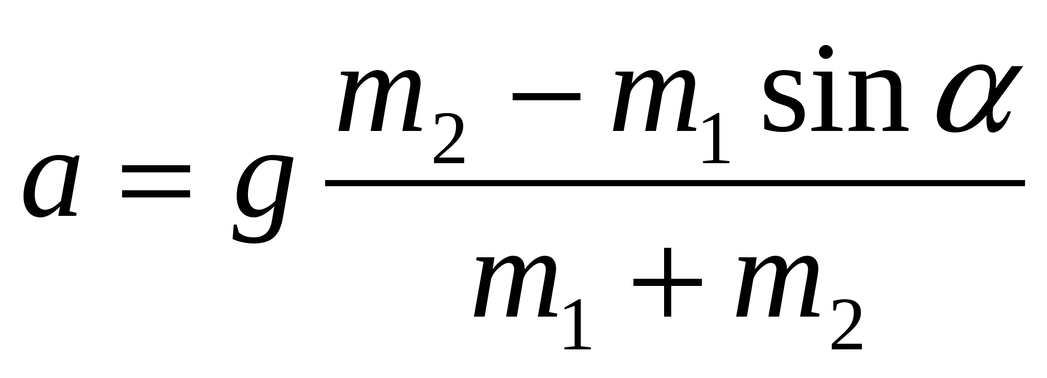

We see that if the value of m 1 sin α were greater than m 2, then the acceleration a would become a negative value. That is, the system would move in the opposite direction (the bar m 1 was lowered, and the load m 2 was raised). The tension force of the thread is found from the last equation:

Consider now a virtual model of a system consisting of two connected bars on an inclined plane.

Figure 13 - Virtual model of connected bodies

In the upper right part of the working field there are regulators with the help of which you can set the system parameters: mass of loads, tilt angle, coefficient of friction. Below are the information windows in which the result of calculations of acceleration, friction force and thread tension is given.buttons "Start", "Reset" and "Help" are located. When you click the "Reset" button, the model returns to its original state. In the center of the window is the working field of the model with the image of an inclined plane and a bar sliding along it. When you press the "Help" button, the student sees equations with which you can independently calculate unknown quantities (Figure 14).

Figure 14 - Menu "Help" model of connected bodies

This model can be used in learning to solve problems for the movement of connected bodies on an inclined plane. The appendix provides examples of tasks that can be solved using this virtual model.

3Practical exercises

In the 2nd section of this work, the basics of the theory of harmonic oscillations and two common cases of bodies of an inclined plane were examined with illustrations from interactive models. In section 3, we will analyze how this model can be used as a virtual laboratory when working with students of a secondary vocational educational institution with a technical profile of training in practical classes. To study mechanical oscillations, 8 hours are allotted, including 1 laboratory work on calculating the acceleration of free fall using a mathematical pendulum (2 hours).

To control the assimilation and understanding of the topic "Mechanical vibrations" by students, it is possible to use a virtual model of a mathematical pendulum. The students were presented with such a model in order to visually demonstrate the principles of the oscillatory process, as well as to observe an example of such a process.

3.1.1 Lab task

As mentioned above, the study of the topic "Mechanical vibrations" involves the implementation of laboratory work, the instructional and technological map of which is given in Appendix 2. An interactive model of a mathematical pendulum is used for admission to practical work or its protection. Appendix 3 contains brief instructions for filling in the table based on the experimental data obtained by the student in the process of working with the model. There are also questions for self-control that will help the student to protect the work. Such an integrated and comprehensive approach will allow the teacher to objectively assess knowledge and significantly save time, which can be more effectively used for individual work and consultations.

3.1.2 Assignment to the model of a mathematical pendulum

The task contains paragraphs describing the instructions for managing the model, a description of the main functions and graphs. It is given in Appendix 4. It helps the trainee understand the purpose of the model and master its adjustments. In addition, the task includes control questions on the topic "Mechanical vibrations" and several computer experiments.

The experiments included in the introductory tasks allow you to delve deeper into the meaning of what is happening on the screen. To perform experiments, it is enough to know the basic formulas of the topic under study. Despite the apparent simplicity, such tasks are very useful, as they allow students to see a live connection between a computer experiment and the physics of the phenomena being studied.

Annex 4 also offers an answer sheet for each introductory task. Recording the received answers in the form allows you to significantly reduce the time of working with a computer model, and makes it easier to check the answers.

3.1.3 "Mechanical vibrations" test

In the course of the work, a theoretical test was applied on the topic "Mechanical vibrations" (Appendix 5).

The purpose of testing: to test the knowledge gained by the trainee in the course of studying the material.

Test control is very important in the pedagogical process. Depending on the results of the control, a decision is made on the need for additional classes and consultations, on providing assistance to underachievers. Answers to the preparation test can be found in Appendix 5.

This closed-type test is criterion-oriented, that is, testing is carried out in order to determine the degree of knowledge of the material and compare results with a well-defined area of ​​\u200b\u200bachievement.

The test consists of 35 tasks of varying complexity. Depending on the purpose of the test, the teacher can choose one or another task.

3.1.4 Outline of lessons "Mechanical vibrations" and "Movement of bodies under the action of several forces"

Annexes 1 and 6 contain lesson notes that can be used in lectures.

3.1.5 Practice-oriented tasks

CONCLUSION

The existing experience has shown that in the formation of professional competencies for future technical specialists, it is effective to use this methodological recommendation and the use of virtual models of physical experiments.

The generated examples of assignments for lectures and practical classes used in training brought positive results. Contributed to strengthening the student's activity approach to learning, motivated him to self-development, including in the field of information technology and deepening knowledge in the physics of natural and man-made processes. It was also noted that when applying these methodological recommendations, students train logic, the difficulties that arise push them to solve problems on their own, which directly contributes to the formation of general and professional competencies necessary for the future technician.

A set of questions for the student, providing the conditions for self-control, will allow an objective assessment of the intermediate and final control of knowledge.

In conclusion, I would like to once again emphasize the importance and necessity of using innovative educational models and technologies when working with students of secondary specialized educational institutions. Since in the process of their application, favorable conditions were created for the differentiation and individualization of training.

LIST OF USED SOURCES

Avanesov V.S. Composition of test tasks / V.S. Avanesov. - M.: Adept, 1998. - 191 p.

Boev V.D., Sypchenko R.P., Computer modeling / V.D. Boev, R.P. Sypchenko. - M.: Publishing house INTU IT.RU, 2010. - 349 p.

Bulavin L.A., Vygornitsky N.V., Lebovka N.I. Computer modeling of physical systems / L.A. Bulavin, N.V. Vygornitsky. - Dolgoprudny: Intellect Publishing House, 2011. - 352 p.

For a physics teacher. The use of a computer in the study of physics. - (Rus.). – URL: http://www. uroki. net/ docfiz/ docfiz27. htm

Maiorov A.N. Tests of school achievements: design, implementation, use. Education and culture / A.N. Mayorov. - St. Petersburg: 1996. - 304 p.

Maiorov A.N. Theory and practice of creating tests for the education system / A.N. Mayorov. - M .: "Intellect-center", 2001. - 296 p.

Minskin E.M. From games to knowledge: a guide for teachers / Minskin E.M. - M.: Enlightenment, 1982. - 192 p.

Teaching physics that develops the student. Book 1. Approaches, components, lessons, tasks / Ed. E. M. Braverman. – M.: Association of Teachers of Physics, 2003. – 400 p.

Samoilenko P.I. Physics for professions of socio-economic and humanitarian profiles: a textbook for the secondary prof. education / P.I. Samoilenko. - 6th ed., erased. - M.: Publishing Center "Academy", 2014. - 469 p.

Firsov A.V. Physics for professions and specialties of technical and natural science profiles: textbook / A.V. Firsov; ed. T.I. Trofimova. - 6th ed., erased. - M.: Publishing Center "Academy", 2014. - 352 p.

ATTACHMENT 1

Plan-summary of the lesson "Mechanical vibrations"

APPENDIX 2

Lab #5

Determination of free fall acceleration using a pendulum.

Objective: determine the acceleration of free fall based on the dependence of the period of oscillation of the pendulum on the suspension on the length of the suspension.

Acquired knowledge and skills:

Time norm: 2 hours

Workplace equipment: tripod with clutch and foot, tape with loops at the ends, a set of weights, a measuring tape with millimeter divisions, an electronic stopwatch

Brief theory

P The period of a mathematical pendulum can be determined from the formula:

(1)

To increase the accuracy of the period measurement, it is necessary to measure the time t of a residually large number N of complete oscillations of the pendulum. Then the period

T=t/N (2)

And the free fall acceleration can be calculated by the formula

Completing of the work:

1. Attach the foot to the top of the tripod shaft. Place the tripod on the table so that the end of the foot protrudes beyond the edge of the table surface. Attach one weight from the set to the foot. The load should hang 3-4 cm from the floor.

2. To record the measurement and calculation results, prepare a table:

experience number

L, m

t, s

t cf, s

T, s

g, m/s 2

3. Measure the pendulum length L with a tape.
4.Prepare the time meter for operation in stopwatch mode.
5. Deviate the pendulum by 5-10 cm and release it.
6. Measure the time t, during which he will make 40 complete oscillations.
7. Repeat the experiment 5-7 times, after which calculate the average time for which the pendulum will make 40 oscillations t cf.
8. Calculate the oscillation period using formula (2).
9. Calculate the free fall acceleration using formula (3).
10. Determine the relative error of the result:

* 100% where g ism - the value of the acceleration calculated as a result of the work done,g– value taken from the directory.

Conclusion:

APPENDIX 3

Assignment to the model of a mathematical pendulum

When completing tasks, you can use the "Help" button.

Set the maximum deflection angle.

Set the maximum length of the pendulum.

Press the "Start" button.

After four complete oscillations, press the Stop button.

Please note that in the process of oscillations, potential energy is converted into kinetic energy and vice versa. In this case, the total energy remains constant.

In the lower left corner of the window are the oscillation counter and the stopwatch. Calculate the period of oscillation in two ways. Use the number of oscillations and the time on the stopwatch to calculate in the first way. For the second - use the Thompson formula. Compare your results.

Acceleration of free fall g for this and subsequent tasks is taken equal to 10 m/s 2 . Round the results to two decimal places. Record the results on the answer sheet.

Under what conditions can the Thompson formula be used?

Knowing the oscillation period, calculate the angular frequency ω 1 .

Calculate the angular frequency ω 2 for the minimum length of the pendulum.

Calculate the swing amplitude for the maximum and minimum pendulum lengths.

Write a solution to the equation of oscillation for the maximum and minimum lengths of the pendulum.

Turn off velocity, kinetic and potential energy graphs.

Compare the displacement versus time plots for the maximum and minimum pendulum lengths.

Write down what increment the phase of the oscillation receives in a time equal to the period of the harmonic oscillation.

Calculate the maximum speed for a pendulum length of 2.5 m and for a length of 1.25 m.

Check your calculations graphically. To do this, turn off the offset plot and activate the speed vs. time plot. Compare the maximum speeds for different pendulum lengths graphically.

Calculate the maximum swing acceleration for the maximum and minimum pendulum lengths. Compare your results.

Activate all charts. Set the maximum length of the pendulum and the maximum deflection angle. Also set the maximum damping decrement.

Press the "Start" button.

Carefully study the plots of displacement, velocity, kinetic and potential energy versus time and the phase portrait.

Please note that in the process of oscillations, potential energy is converted into kinetic energy and vice versa. In this case, the total energy decreases exponentially.

Calculate the period of oscillation using Thompson's formula.

Compare the resulting oscillation period with the period obtained in
paragraph 7.

Knowing the oscillation period, calculate the angular frequency ω.

Calculate the maximum amplitude of the oscillation.

Press the "Start" button again. After one full swing, press the Stop button.

Calculate the maximum amplitude of the second oscillation, knowing the damping factor and the timer.

Check your calculations by clicking the "Calculate" button.

Write the solution to the equation of oscillation for the maximum length of the pendulum.

Calculate the maximum speed and acceleration values ​​for the time that the timer shows.

Answer form for the task to the model of a mathematical pendulum
FULL NAME. student ___________________________________________________

1. Oscillation period in 1 case __________________ sec.
   Oscillation period in case 2 _________________ sec.

1. Thompson's formula can be used when ______________________________________________________________________________________________________________________________

   ω 1 \u003d _______________ rad / sec.

   ω 2 \u003d _______________ rad / sec.

   BUT 1 = _______________ m. BUT 2 = _______________ m.

   __________________________________________________________________________________________________________________________________________________________________________________

   With an increase in the length of the pendulum ________________________ ________________________________________________________________

   ______________________________________________________ ________________________________________________________________

   υ 1 \u003d _______________ m / s. υ 2 \u003d _______________ m / s.
   With an increase in the length of the pendulum, the speed ___________________________ ________________________________________________________________

   a 1 \u003d _______________ m / s 2. a 2 \u003d _______________ m / s 2.
   With an increase in the length of the pendulum ________________________________________________ ________________________________________________________________

   T= ___________________ sec.

   With an increase in the attenuation coefficient, the period of the mathematical pendulum ______________________________________ ____________________________________________________________

   ω \u003d ___________________ rad / sec.

   BUT 1 = _______________ m.

   BUT 2 = _______________ m.

   ______________________________________________________________________________________________________________________

   υ = _______________ m/s. a\u003d _______________ m / s 2.

APPENDIX 4

Assignment for independent work

Completed tables are handed over by students in notebooks for laboratory work. For filling, an interactive model of a mathematical pendulum is used.

1 A) By setting the slider to 2-3 different positions in the lines "Angle of deflection" and "Length of the pendulum", fill in the table. At the same time, leave the slider in the line "Attenuation coefficient" in the zero position.

Deflection angle

pendulum length

Period

corner frequency

Speed mx

Acceleration max

C) Find the maximum values ​​of kinetic and potential energy. Draw a graph of energy versus time.

C) Make a conclusion about the type of mechanical vibrations.

2 A) By setting the slider in 2-3 different positions in the lines "Angle of deviation", "Length of the pendulum" and "Damping coefficient", fill in the table.

Deflection angle

pendulum length

Attenuation factor

Period

corner frequency

Speed mx

Acceleration max

B) Calculate the indicated values ​​yourself and compare with those given in the calculations. Bring the calculations in your notebook and draw a phase portrait.

Questions for self-control:

What vibrations are called harmonic? Give examples of harmonic oscillations.

Define the following characteristics of a harmonic oscillation: amplitude, phase, initial phase, period, frequency, cyclic frequency.

Derive the differential equation of harmonic oscillations and write its solution.

How do the kinetic and potential energies of a harmonic oscillation change with time? Why does the total energy of a harmonic oscillation remain constant?

Derive a differential equation describing damped oscillations and write its solution.

What is the logarithmic damping factor?

What is resonance? Draw a plot of the amplitude of the forced oscillations versus the frequency of the driving force when this force is a simple harmonic function of time.

What is self-oscillation? Give examples of self-oscillations.

APPENDIX 5

test on the topic "Mechanical vibrations"

1. 1. What is called a mathematical pendulum?

A rigid body suspended from a spring

A material point suspended on a weightless inextensible thread

A rigid body suspended from a weightless inextensible thread

Any rigid body that oscillates about its equilibrium position

1. 1. What is a wave front?

Geometric locus of points oscillating in one phase

Locus of points oscillating with different phase

Geometric locus of points to which oscillations reach by time t

The locus of points on the wave surface

1. 1. What is called the amplitude of oscillations?

Maximum period value

The maximum value of the fluctuating quantity

The maximum frequency value at which the resonance phenomenon is observed

Minimum value of fluctuating quantity

1. 1. What is called free vibration?

Oscillations that are made due to the initially imparted energy with the subsequent absence of external influences on the oscillatory system

Oscillations that occur due to the energy of external influences on the oscillatory system

4) Any fluctuations occurring in nature

1. 1. What is a harmonic oscillation?

Any fluctuations found in nature

Processes that are characterized by a certain repeatability in time

Oscillations in which the oscillating quantity changes with time according to the law of sine or cosine

Oscillations that occur due to the total energy of external influences and natural oscillations of the system

1. 1. What is the oscillation frequency?

The time it takes for one complete oscillation

The total number of complete oscillations made in time t

Time for a quarter swing

The number of complete oscillations per unit of time

1. 1. What is called the period of oscillation?

The time it takes for vibrations to completely die out

Time of one full oscillation

A value equal to the reciprocal of the number of oscillations

Logarithm of the ratio of successive amplitudes

1. 1. What is the oscillation phase?

The value that is under the sign of sine or cosine and determines the instantaneous value of the period of oscillation

The value that is under the sign of sine or cosine and determines the duration of a complete oscillation

A value that is under the sign of sine or cosine and determines the instantaneous state of the oscillatory system.

The value under the sine or cosine sign and which determines the maximum deviation from the equilibrium position

1. 1. What increment does the phase of the oscillation receive in a time equal to the period of the harmonic oscillation?

1. 1. At what maximum deflection angle can we assume that the mathematical pendulum still performs harmonic oscillations?

Decreases

is increasing

Doesn't change

Changes slightly

1. 1. How do the frequencies of damped and undamped oscillations correlate?

Frequencies are equal

The frequency of undamped oscillations is less

The frequency of damped oscillations is less

The frequency of damped oscillations is greater

1. 1. According to what law does the amplitude of damped oscillations decrease?

Linear

According to the law of cosine

By quadratic

Exponential

1. 1. What is the reduced length of a physical pendulum called?

The length of the whole pendulum

The length of a mathematical pendulum whose period of oscillation is equal to the period of oscillation of a physical pendulum

The length of the mathematical pendulum

1/2 the length of a mathematical pendulum

1. 1. What formula can be used to calculate the acceleration of free fall using a mathematical pendulum?

1. 1. The figure shows the graphs of displacement, velocity, potential and kinetic energies versus time. What is the color of the graph of kinetic energy versus time?

3. Violet

1. 1. The figure shows the graphs of displacement, velocity, potential and kinetic energies versus time. What is the color of the offset vs. time graph?

3. Violet

1. 1. The figure shows the graphs of displacement, velocity, potential and kinetic energies versus time. Which dependency is shown in yellow?

Time offset dependencies

Speed ​​versus time

Dependences of kinetic energy on time

Potential energy versus time

1. 1. What is a phase portrait?

Offset versus time plot

Graph of speed versus time

Displacement versus speed plot

Graph of total energy versus time

1. 1. The figure shows a graph of the phase portrait of the oscillation. Determine what the swing is.

Harmonic damping

Harmonic sustained

Non-harmonic damped

Non-harmonic undamped

Answers to the test "Mechanical vibrations"

Number
question

Number
correct answer

Number
question

Number
correct answer

Number
question

Number
correct answer

3) Support reaction force ___________________________________________________________________________________________________________________________________________________________________________________________________________________________

4) N ​​= ____________________

5) Coefficient of friction - __________________________________________________________________________________________________________________________________________________________________________________________________________

6) µ=_____________________

7) Maximum angle of inclination (limiting angle), α max ______________________________________________

8) Acceleration, a \u003d ________________________________________

1. Arrange the regulators in arbitrary positions and write down the initial data in the table.

   Press the "Start" button and watch the movement of the bar

   Write down the value of the friction force, the reaction force of the support, the acceleration of the body, located in the scoreboard on the working field of the model.

   Calculate independently the value of the friction force, the reaction force of the support, the acceleration of the body, as well as the maximum angle of inclination of the plane.

Tilt angle, α, deg

friction coefficient,
µ

m , kg

Values ​​computed by the model

Values ​​computed by the student

Limit angle, α max

Friction force, F tr, N

Accelerationa, m/s 2

Support reaction force, N , N

Friction force, F tr, N

Accelerationa, m/s 2

Support reaction force, N , N

Plot velocity versus time V(t):

Conclusion_________________________________________________________________________________________________________________________________________________________________________________________________________________________________________________________________________________________________

Study of physical models Prepared by: Anastasia Kukleva

Modeling is a means of studying a system by replacing it with a system (model) that is more convenient for research, preserving the properties of interest to the researcher. Modeling is the construction (or selection) and study of models in order to gain new knowledge about objects. A model is an object of any nature that is capable of replacing the object under study in the properties of interest to the researcher (for example, a globe is a model of the Earth). Description of the object - a set of information about the system under study and the conditions under which it is necessary to conduct a study.

Classification (proposed by VA Venikov) Logical models Logical models are created on the basis of reasoning. Any person, before performing some action, builds a logical model. The correctness of the logical model shows time. Models of this type not always known to us have been confirmed. The advantage of logical models is the presence in all other types of models. Physical Models Models that are physically similar to a real system. The main difference between physical models is the physical similarity of the most important properties under study. The most striking examples of physical models are children's toys. Another example - when designing a car, designers build a plasticine physical model of the future product. The advantage of this type of model is the highest degree of visibility of the results. Mathematical models A mathematical model is a description of the system under study, strictly formalized in the language of mathematics. The advantage is a strictly formalized proof and validity of the results obtained. (for example, a system of linear equations is a method for solving it). This type of modeling is currently decisive in system research. Simulation (computer) modeling Simulation modeling is a numerical experiment with mathematical models of the elements of the system under study, combined at the information level. Simulation models can contain not only mathematical models of the elements of the system under study, but also physical models. (for example, a trainer).

Study of physical models. Movement under the influence of gravity is well known. This is the fall of a body from a certain height, and the movement of a body thrown at an angle to the horizon, etc. If in such problems the force of air resistance is not taken into account, then all the listed types of motion are described by known formulas. But problems in which air resistance is taken into account are no less interesting.

Task Movement of the parachutist.

I stage. Problem statement DESCRIPTION OF THE PROBLEM When falling to the ground, a parachutist experiences the action of gravity and air resistance. It has been experimentally established that the resistance force depends on the speed of movement: the greater the speed, the greater the force. When moving in the air, this force is proportional to the square of the speed with some drag coefficient k, which depends on the design of the parachute and the weight of the person. What should be the value of this coefficient in order for the skydiver to land on the ground at a speed of no more than 8 m / s, which does not pose a health hazard? Determine the goals of modeling and formalize the task.

II stage. Model development INFORMATION MODEL Build your own information model. MATHEMATICAL MODEL The figure shows the forces acting on the skydiver. According to Newton's second law, motion under the action of forces can be written as equality.

We project this equality onto the axis of motion, substitute the expression for the air resistance force. We obtain a formula for calculating the acceleration

We will calculate the speed and distance that the skydiver flew at regular intervals Δt. The formula for calculating the moments of time is: ti+1=ti+Δt We will also assume that the acceleration is constant and equal to ai on each interval. The formula for calculating the acceleration is: where Vi is the speed at the beginning of the interval (V0 is the initial speed).

The speed at the end of the interval (and, accordingly, at the beginning of the next one) is calculated by the formula of uniformly accelerated motion.

COMPUTER MODEL For simulation, we will choose a spreadsheet environment. In this environment, the information and mathematical model are combined into a table that contains three areas: initial data; intermediate settlements; results.

III stage. computer experiment

Formal model To formalize the model, we use the formulas of uniform and uniformly accelerated motion known from the course of physics.

Thank you for your attention!!!